Data Source Paper.
Botero-Valencia et al., MDPI Data — "Exploring Spatial Patterns in Sensor Data for Humidity, Temperature, and RSSI Measurements."
Raw dataset available at: osf.io/zbn8w
All experiments use data collected from Lab 1, a real indoor office environment
instrumented with a wireless sensor network of 13 IoT nodes.
Each node logs temperature, relative humidity, and RSSI at approximately 10-second intervals.
The dataset covers 40 days of continuous measurements,
providing both short-term dynamics and longer seasonal drift.
13
Sensors
40
Days
~10s
Raw Sample Rate
3
Channels (T, RH, RSSI)
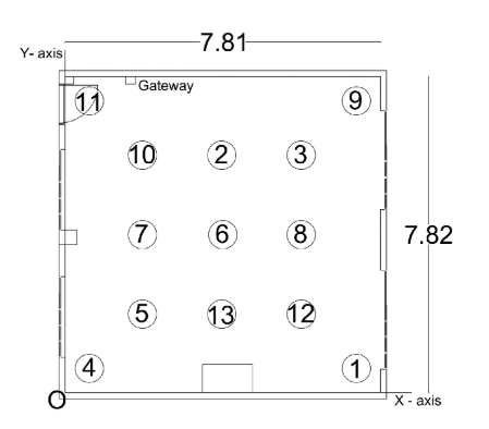
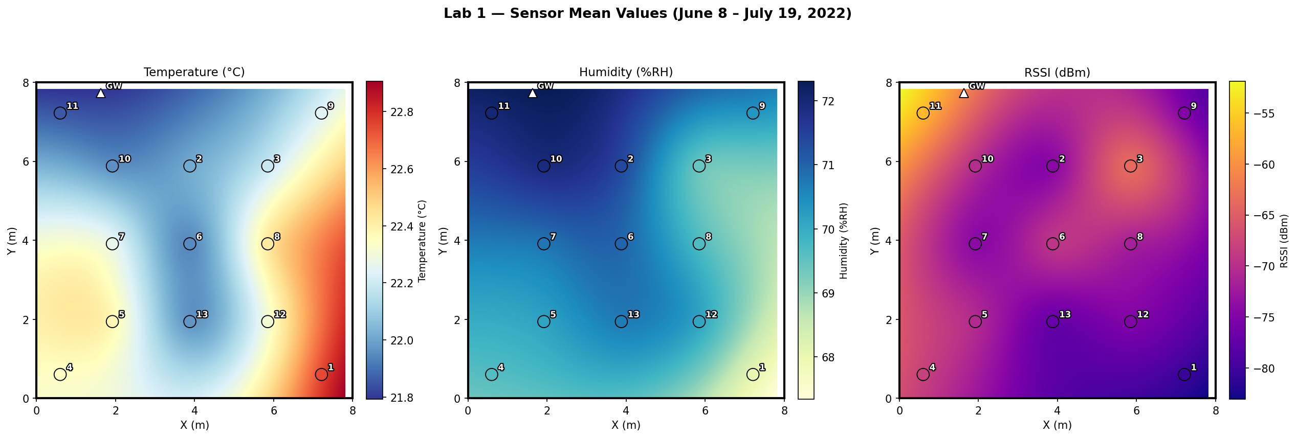
Lab 1 Layout. Floor plan of the instrumented room showing walls, furniture, and general sensor deployment zones.Sensor Positions. Exact (x, y) coordinates of all 13 sensor nodes used as the trunk-net inputs for DeepONet.
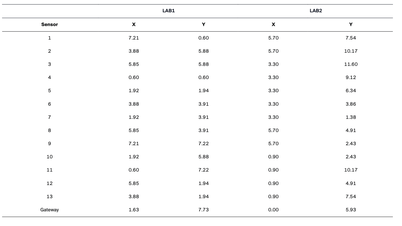
Figure 1-3 — Sensor 6 Temperature Time Series. Raw 10-second measurements (gray) overlaid with 5-minute resampled means (blue). The high-frequency noise present in the raw data motivates our resampling and filtering investigations.Figure 1-4 — Spatial Field Heatmaps. Mean Temperature (°C), Relative Humidity (%), and RSSI (dBm) across the room, interpolated from the 13 sensor positions using RBF thin-plate spline interpolation. These maps reveal the spatial gradients the model must learn to reproduce.
2
Model Architecture
Operator Network & DeepONet
What is an Operator Network?
Standard neural networks map one fixed-size vector to another. An operator network
goes one level higher: it learns a mapping between functions.
In our case, the input function is the temperature field observed at 12 sensor locations at a given time,
and the output function is the full spatial temperature field — so we can query it at any (x, y) coordinate in the room.
This means the model generalises to locations where we have no sensors,
effectively reconstructing the continuous temperature field from sparse measurements.
How DeepONet Works
DeepONet (Deep Operator Network, Lu et al. 2021) implements this idea with two coupled sub-networks:
Branch Network
Encodes the input function — the sensor readings at a fixed set of measurement locations. Produces a latent vector that summarises the current state of the room.
Trunk Network
Encodes the query location — the (x, y) coordinate where we want to predict the temperature. Produces a basis vector for that position.
The final prediction is the dot product of the branch and trunk outputs
(plus a bias), giving a single temperature value at the queried location.
By sweeping the query over a dense grid, we reconstruct the entire 2D temperature field.
Our Architecture
INPUT ├─ Branch input: 12 sensor temperatures at time t (shape: [12]) └─ Trunk input: (x, y) query coordinate (shape: [2])
BRANCH NET (MLP) 12 → 128 → 128 → 128 → p (ReLU activations) └─ output: latent vector b ∈ ℝp
TRUNK NET (MLP) 2 → 128 → 128 → 128 → p (ReLU activations) └─ output: basis vector t ∈ ℝp
OUTPUT T̂(x,y) = b · t + bias (dot product + scalar bias)
TRAINING STRATEGY ├─ Sensor 7 withheld from branch input (used as test target) ├─ Loss: MSE on withheld sensor temperature └─ Optimiser: Adam, lr=1e-3, cosine annealing
Why Sensor 7?
Sensor 7 is withheld from the branch input in all experiments. The model sees only the other 12 sensors during inference and must reconstruct the temperature at Sensor 7's (x, y) location. This simulates a real-world scenario where a sensor goes offline or is not deployed.
3
Baseline Results
Raw 10s Data vs. 5-Min Resampled Data
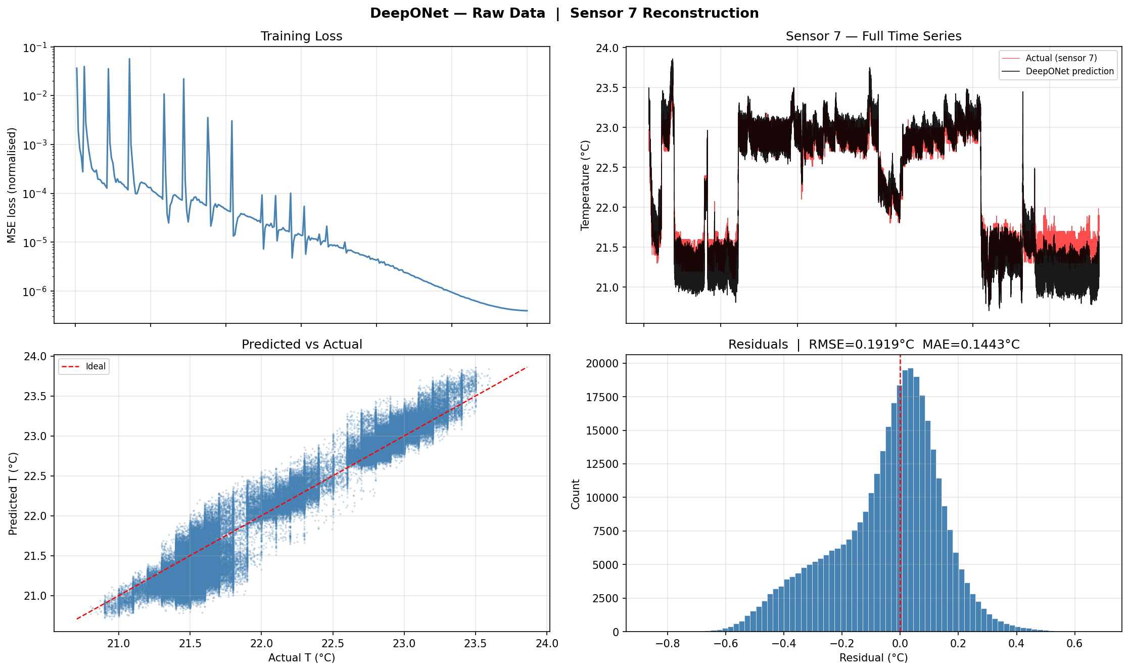
As a first experiment we trained two identical DeepONet models —
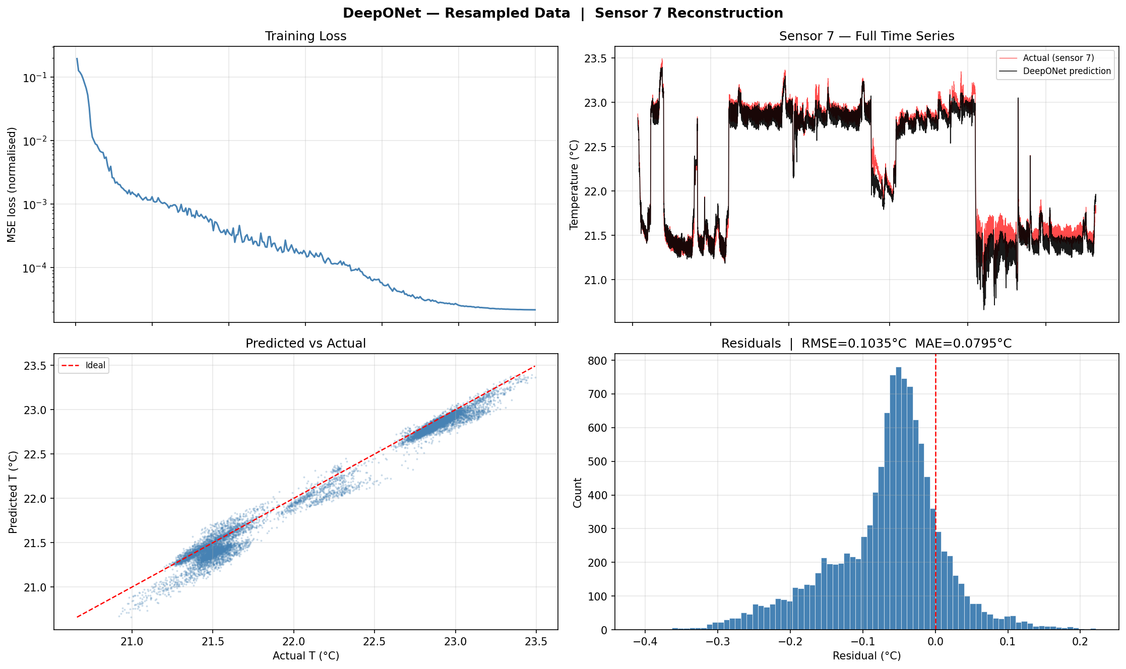
one on the raw 10-second data and one on 5-minute mean-resampled data —
to understand whether input noise level affects reconstruction accuracy.
Raw (10s) Training. Loss curve, predicted vs. actual time series for Sensor 7, scatter plot, and residual distribution for the model trained on high-frequency raw data.5-Min Resampled Training. Same four diagnostics for the model trained on 5-minute averages. Noise reduction in the input leads to visibly smoother predictions and lower residuals.
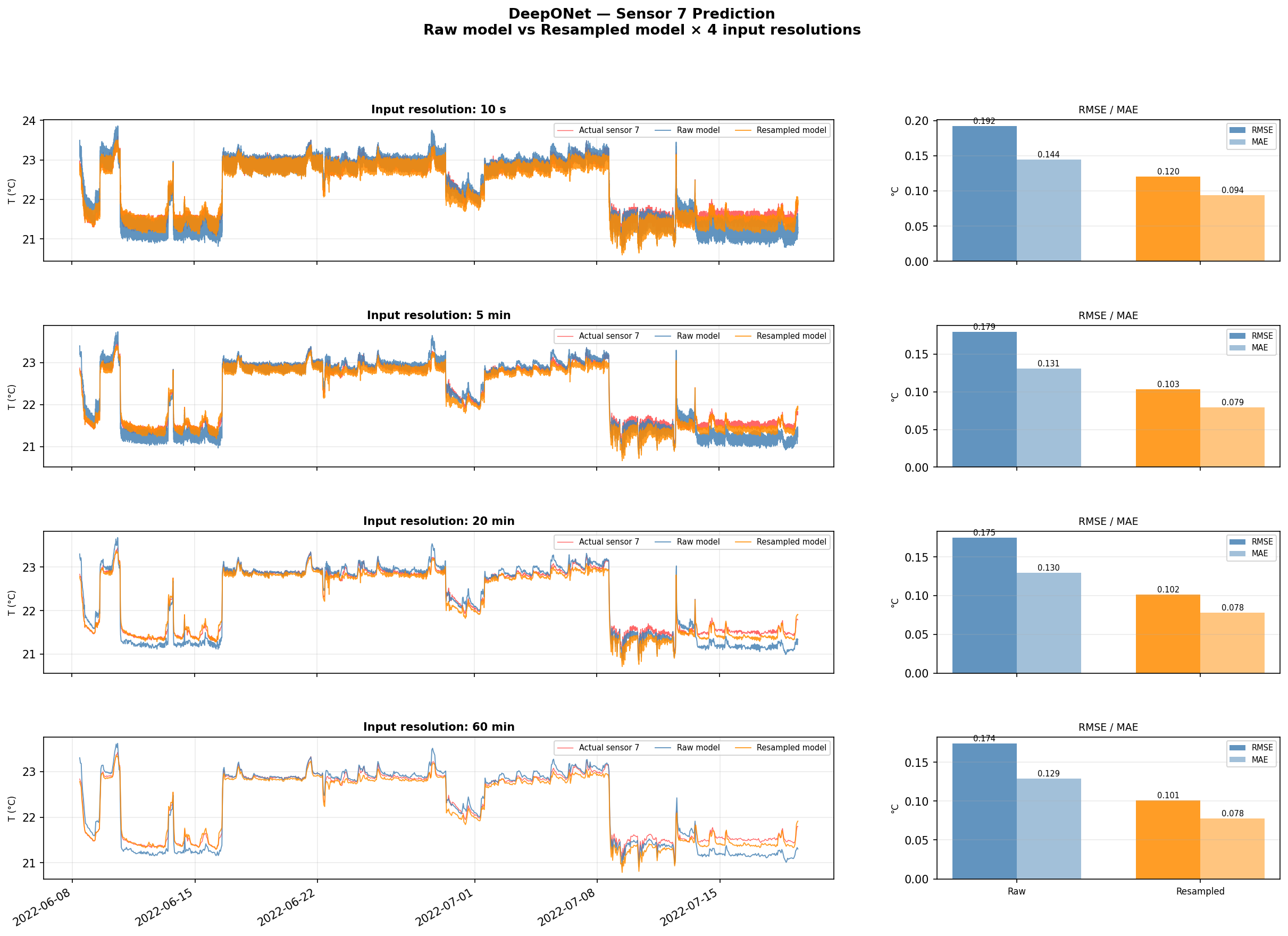
Figure 3-3 — Multi-Resolution Prediction Comparison. Both trained models are evaluated at four input resolutions (10s, 5min, 20min, 60min). Each row shows the predicted vs. actual time series for Sensor 7, with RMSE and MAE bar charts on the right. The resampled model generalises more robustly across resolutions.
4
Noise Analysis
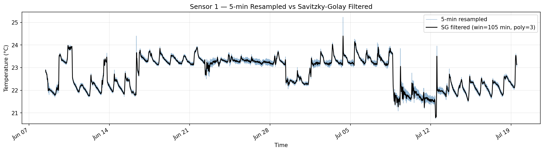
Noisy Data & Savitzky-Golay Filtering
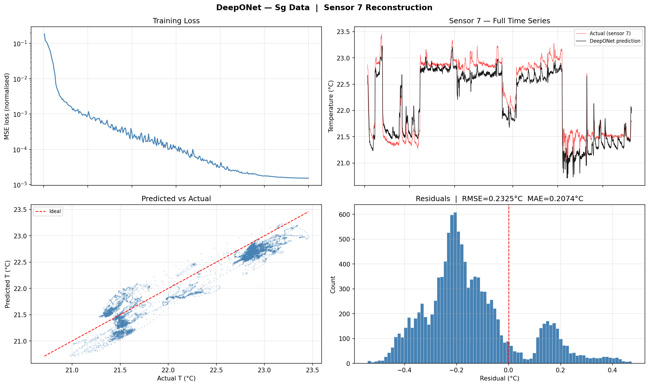
To better understand the effect of noise, we compared the raw 5-minute data with
a smoothed version produced by a Savitzky-Golay (SG) filter,
then trained a DeepONet on the filtered signal.
What is a Savitzky-Golay Filter?
The Savitzky-Golay filter is a digital smoothing technique that fits a low-degree polynomial
to a sliding window of data points using least squares, then replaces each point with the
polynomial's value at that position.
Unlike a simple moving average, it preserves the shape of peaks and edges —
important for temperature data where ramp-up and cool-down dynamics carry physical meaning.
We use a window of 21 points (~105 minutes) and polynomial order 3.
Figure 4-2 — Sensor 1: 5-min Resampled vs. SG-Filtered. The SG filter removes short-term fluctuations while following the overall temperature trend faithfully, including daily cycles.Figure 4-3 — DeepONet Trained on SG-Filtered Data. Loss curve, time series, scatter, and residuals for the model trained on smoothed inputs. Training is more stable and the residual distribution is tighter than the raw model.
5
Feature Engineering
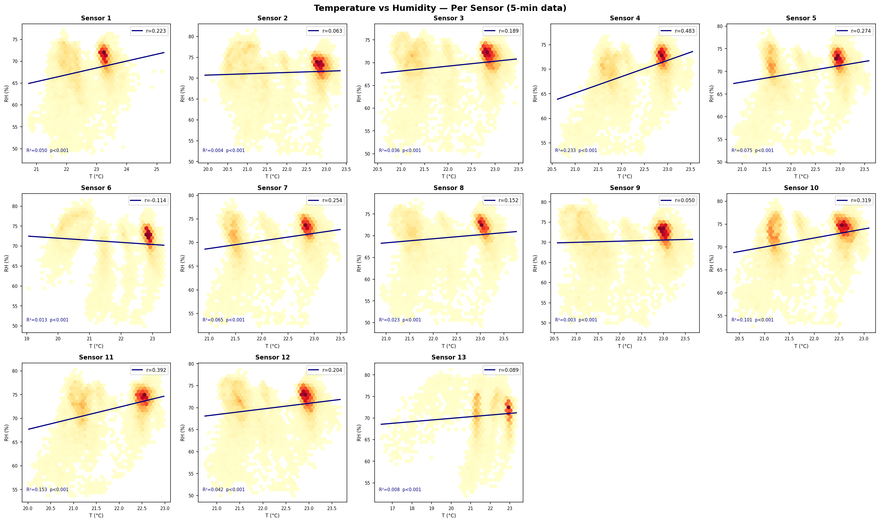
Humidity–Temperature Correlation & PCA Feature
Temperature and humidity in a room are physically coupled — HVAC systems control both,
and occupancy affects both. We investigated whether humidity carries additional information
that could improve temperature reconstruction.
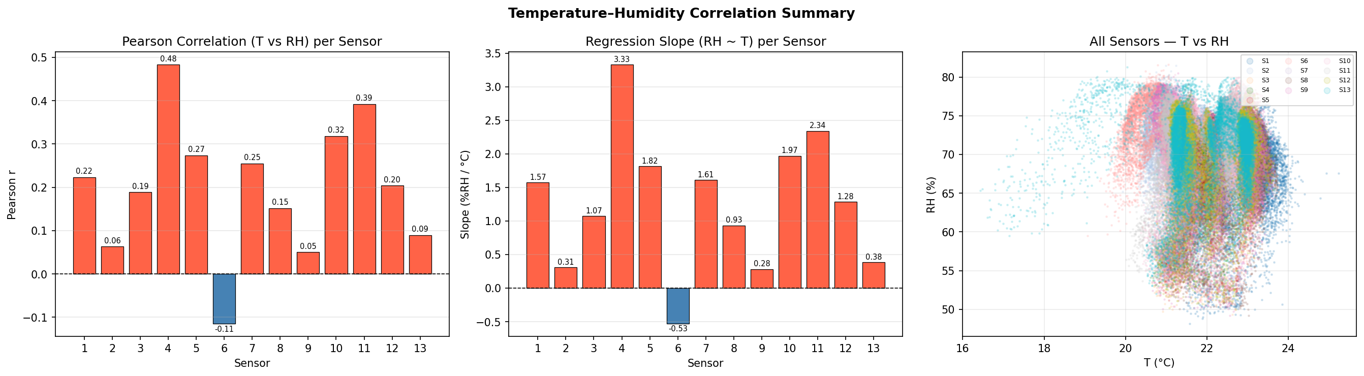
Figure 5-1 — Per-Sensor T vs. RH Scatter. Linear regression fit for each of the 13 sensors individually. Most sensors show a strong negative correlation (higher temperature → lower relative humidity).Figure 5-2 — Pearson Correlation Summary. Bar chart of Pearson r per sensor and joint scatter. The consistently negative r values confirm a room-wide anti-correlation between T and RH.
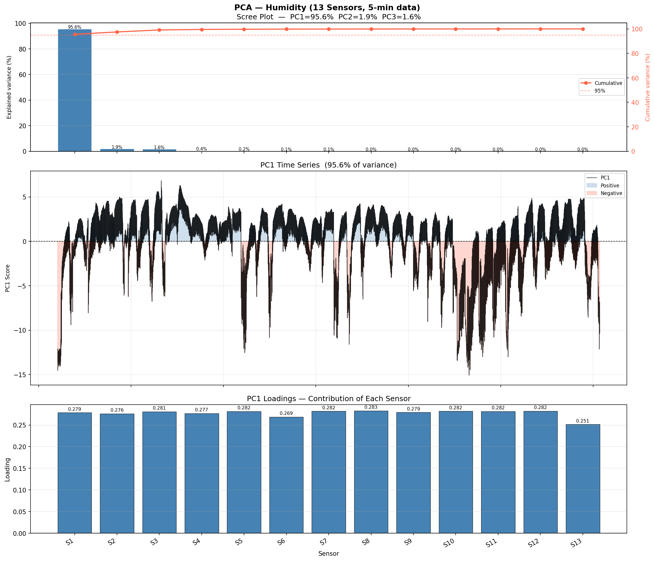
Figure 5-3 — PCA on Humidity Signals. Scree plot (left) and PC1 time series (right). PC1 captures the dominant shared variance across all 13 humidity sensors, essentially tracking the room-level humidity mode.
What is PCA?
Principal Component Analysis (PCA) is a linear dimensionality reduction technique.
Given N correlated signals (here: 13 humidity time series), PCA finds a set of orthogonal
directions — principal components — ordered by the amount of variance they explain.
PC1 is the first principal component:
a single time series that is the linear combination of all 13 humidity channels
that explains the most variance. Because all sensors are in the same room and
strongly correlated, PC1 alone captures the dominant room-wide humidity pattern,
compressing 13 channels into 1 without losing much information.
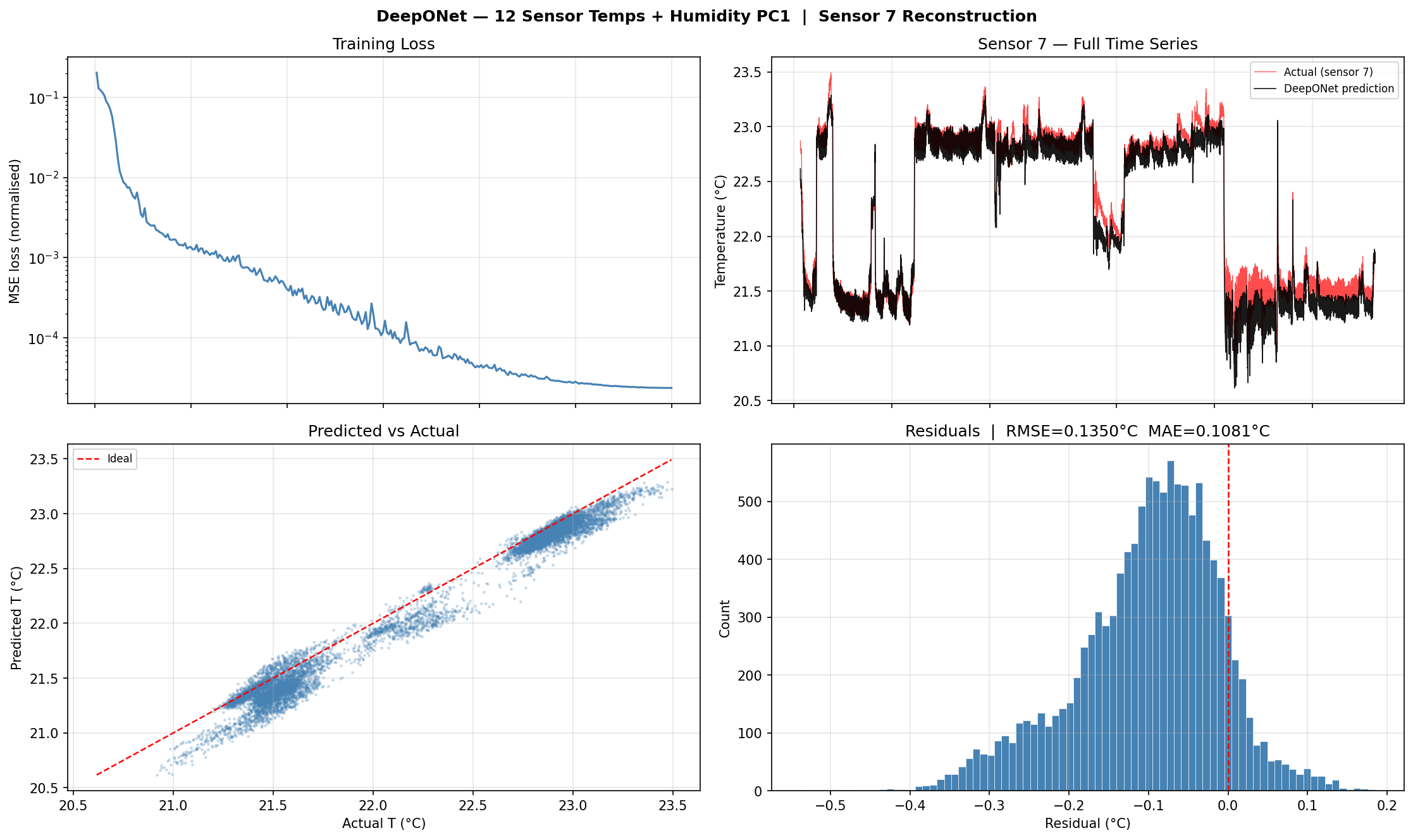
Adding Humidity PC1 to the Model
The branch network input is extended from 12 to 13 features
by appending the humidity PC1 value at each timestep alongside the 12 sensor temperatures.
Everything else (trunk net, training procedure, withheld sensor) stays the same.
Figure 5-5 — DeepONet with Humidity PC1 as Extra Input. Adding the humidity principal component improves the model's ability to track abrupt temperature changes, reducing residual spread.
6
Sequence Modelling
LSTM Branch Network
The baseline DeepONet branch network processes a single timestep snapshot of the sensor array.
It has no memory of past states. To exploit temporal dependencies in the temperature signal,
we replace the MLP branch with a Long Short-Term Memory (LSTM) network
that encodes a sliding window of recent history.
What is LSTM?
LSTM (Long Short-Term Memory) is a type of recurrent neural network designed to learn
long-range dependencies in sequential data. Unlike a simple RNN, an LSTM cell maintains
two state vectors: a cell state (long-term memory)
and a hidden state (short-term output).
Three gates — input, forget, and output — learn to write, erase, and read from the cell state,
preventing the gradient from vanishing over long sequences.
This makes LSTMs well-suited for temperature time series, where a room's thermal inertia
means the current temperature depends on what happened in the past hour or more.
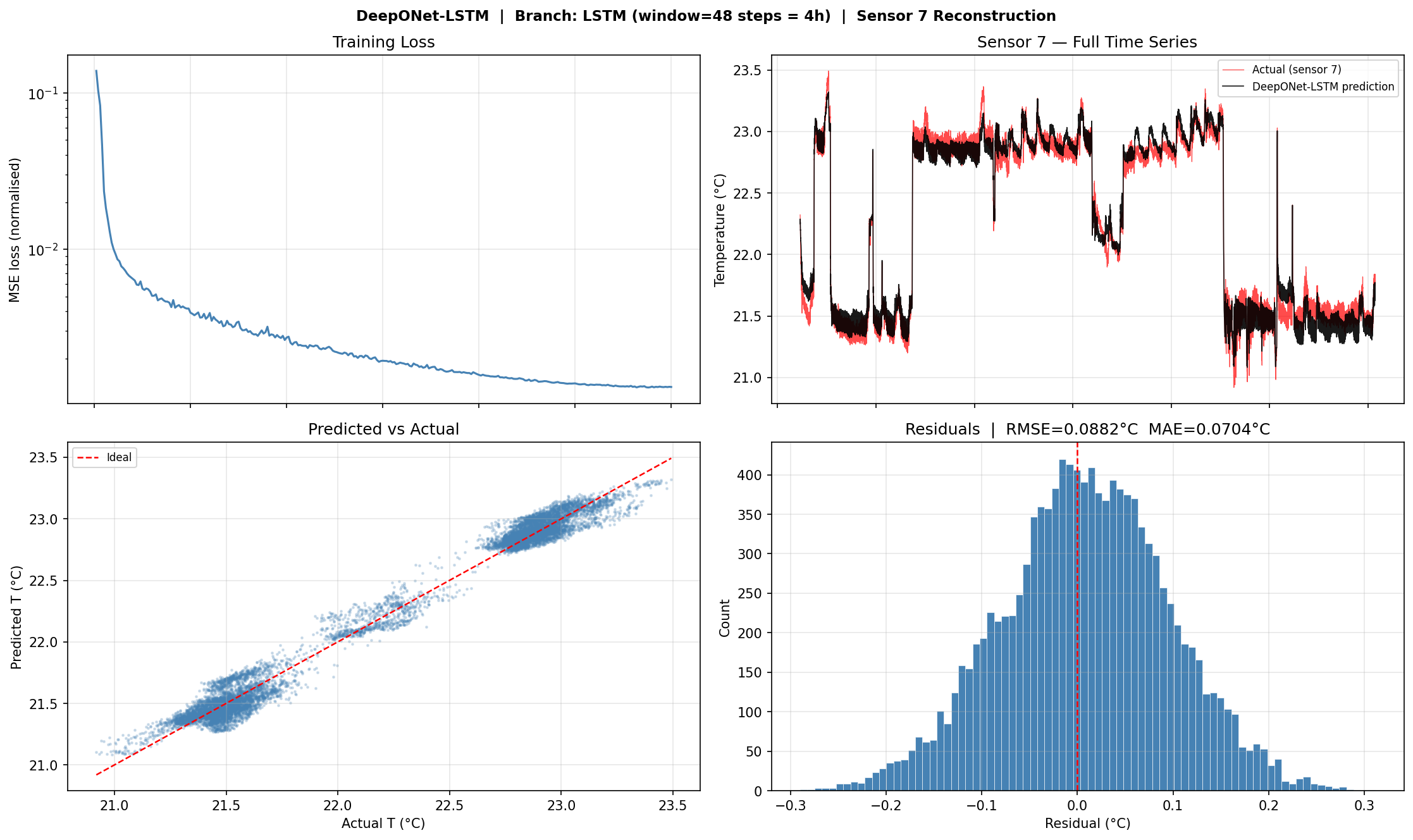
LSTM Branch Architecture
LSTM BRANCH NET ├─ Input: sliding window of 48 timesteps × 12 sensors (= last 4 hours at 5-min resolution) ├─ LSTM Layer 1: hidden_size = 128, dropout = 0.1 ├─ LSTM Layer 2: hidden_size = 128 ├─ Take last hidden state h_T ∈ ℝ128 └─ Linear projection: 128 → p (same p as trunk net output)
TRUNK NET (unchanged MLP) 2 → 128 → 128 → 128 → p
OUTPUT T̂(x,y) = b_LSTM · t_trunk + bias
KEY DIFFERENCE vs. BASELINE Branch sees 48 past timesteps instead of just the current snapshot. The LSTM learns which part of recent history matters most.
Figure 6-2 — DeepONet-LSTM Results. Loss curve, predicted vs. actual time series for the withheld Sensor 7, scatter plot, and residual distribution. The LSTM branch captures temporal dynamics that the snapshot-based MLP branch misses, leading to improved tracking of temperature ramps.
A purely data-driven model can fit sensor observations accurately but has no guarantee that its
spatial temperature field obeys the governing equations of heat transfer.
To constrain the solution to physically plausible dynamics, we add a
PDE residual loss derived from the advection-diffusion-source equation
for indoor thermal fields. The key departure from an RC-circuit approach is that this formulation
is fully continuous in space — it reasons about the temperature field at every point in the room,
not just at sensor locations.
Why Advection-Diffusion instead of a Lumped RC Model?
An RC network is a lumped model: it treats the room as a small number of discrete
zones connected by resistors. It cannot represent how heat spreads continuously across the
floor plan. The advection-diffusion PDE operates on the continuous spatial field
T(x, y, t) that the DeepONet trunk already represents, so the physics loss
directly penalises the network output at any queried coordinate — including the withheld
Sensor 7 location.
Governing Equation
The temperature field satisfies the following PDE at every interior point of the room:
ADVECTION-DIFFUSION-SOURCE PDE
∂T/∂t + v(x,y) · ∇T = α ∇²T + S(T̄, x, y)
where: T(x,y,t) = temperature field at position (x,y) at time t v(x,y) = spatially-varying air velocity field (learned by v-net) α = thermal diffusivity scalar (learned, log-space for positivity) S(T̄, x, y) = spatially-varying heat source/sink (learned by source-net) T̄ = mean sensor temperature (scalar context for S)
TOTAL TRAINING LOSS L = λ_data · L_data + λ_pde · ( L_pde + λ_div · L_div + λ_noslip · L_noslip + λ_sparse · L_sparse + λ_neumann · L_neumann )
Approximated by a finite difference between consecutive 5-minute timesteps:
model(ut+1, xy) − model(ut, xy).
Both evaluations share the same spatial coordinates; only the branch input changes.
∇T and ∇²T — Spatial Derivatives
Computed via automatic differentiation through the SIREN trunk with respect
to the input coordinates (x, y). The SIREN activation (sin(ω₀··)) guarantees
non-vanishing second derivatives everywhere, keeping the Laplacian ∇²T meaningful.
ω₀ = 5 is used (reduced from the standard 30) since thermal fields are spatially smooth —
large ω₀ causes ∇²T ~ ω₀² blow-up in the PDE residual.
Learned Physics Sub-networks
V-NET — Spatially-Varying Velocity Field Input : (x, y) [normalised room coordinates ∈ [0,1]²] Hidden : Linear(2→16) → Tanh → Linear(16→2) Output : (v_x, v_y) [air velocity at each point]
A global scalar velocity cannot represent AC-driven circulation patterns.
The v-net learns the full 2-D velocity field from data.
Kept shallow (1 hidden layer, width 16) to prevent memorising PDE residuals.
Uses only the mean temperature T̄ (not all 12 sensor readings) as temporal context.
Giving the net all 12 readings allows it to reconstruct ∂T/∂t exactly and zero the PDE
residual without learning any physics — a known failure mode called the "source fudge factor."
THERMAL DIFFUSIVITY α α = exp(log_α) — single learnable scalar, initialised at exp(−2) ≈ 0.135
Collocation Strategy
The PDE residual is evaluated at 512 collocation points per training step,
split equally between:
50 % — Sensor Locations
Randomly sampled from the 12 training sensor coordinates.
The data loss anchors the field here, so the PDE is better conditioned at these points.
50 % — Random Interior
Uniformly sampled from the room interior [0,1]².
These enforce the PDE in regions with no sensor, including the neighbourhood
of withheld Sensor 7.
Boundary Condition Losses
Without geometric constraints, spatially-varying MLPs can learn degenerate solutions —
for example, inventing wind that blows through solid walls, or room-wide heat sinks that
absorb the entire PDE residual. Four additional loss terms enforce real-world geometry:
Fix 1 — No-Slip Boundary Condition
L_noslip = ‖v(x_wall)‖²
Air velocity must be zero at solid walls. 64 points are sampled on each of the four
walls at every training step and the v-net output is penalised directly.
This prevents the learned circulation from passing through walls.
Fix 2 — L1 Sparsity on Source
L_sparse = mean(|S(x,y)|)
Real heat sources are localised (AC vents, windows).
L1 on the source output pushes S to exactly zero for most of the room,
forcing the network to concentrate heating/cooling into a small distinct region
rather than spreading a diffuse bias across the entire field.
Fix 3 — Reduced Network Capacity
v-net and source-net are deliberately shallow (1 hidden layer) and narrow
(width 16 and 32 respectively). A deeper, wider network has enough capacity to
memorise the PDE residual as a function of its inputs — effectively becoming
another fudge factor. Reducing capacity forces the networks to learn smooth,
generalisable spatial patterns instead.
Fix 4 — Neumann (Insulated Wall) Condition
L_neumann = (∂T/∂n)2 at walls
Concrete walls have low thermal conductivity, so the normal heat flux at the
perimeter is approximately zero: ∂T/∂n ≈ 0.
The normal gradient of T is computed via autograd at 64 wall points per wall
and penalised. This prevents the temperature field from developing sharp gradients
at the room boundary.
Key Design Principle — The Blind Inverse Problem
The exact AC vent locations, airflow rates, and occupancy patterns are unknown.
Rather than prescribing these from engineering drawings, the model
discovers them from data subject to physical constraints.
The no-slip and Neumann boundary conditions act as geometric priors that rule out
unphysical solutions, while the L1 sparsity and reduced capacity prevent the physics
sub-networks from finding degenerate mathematical shortcuts.
The result is a spatial field that is not only accurate at sensor locations but
physically consistent everywhere in the room.
Results
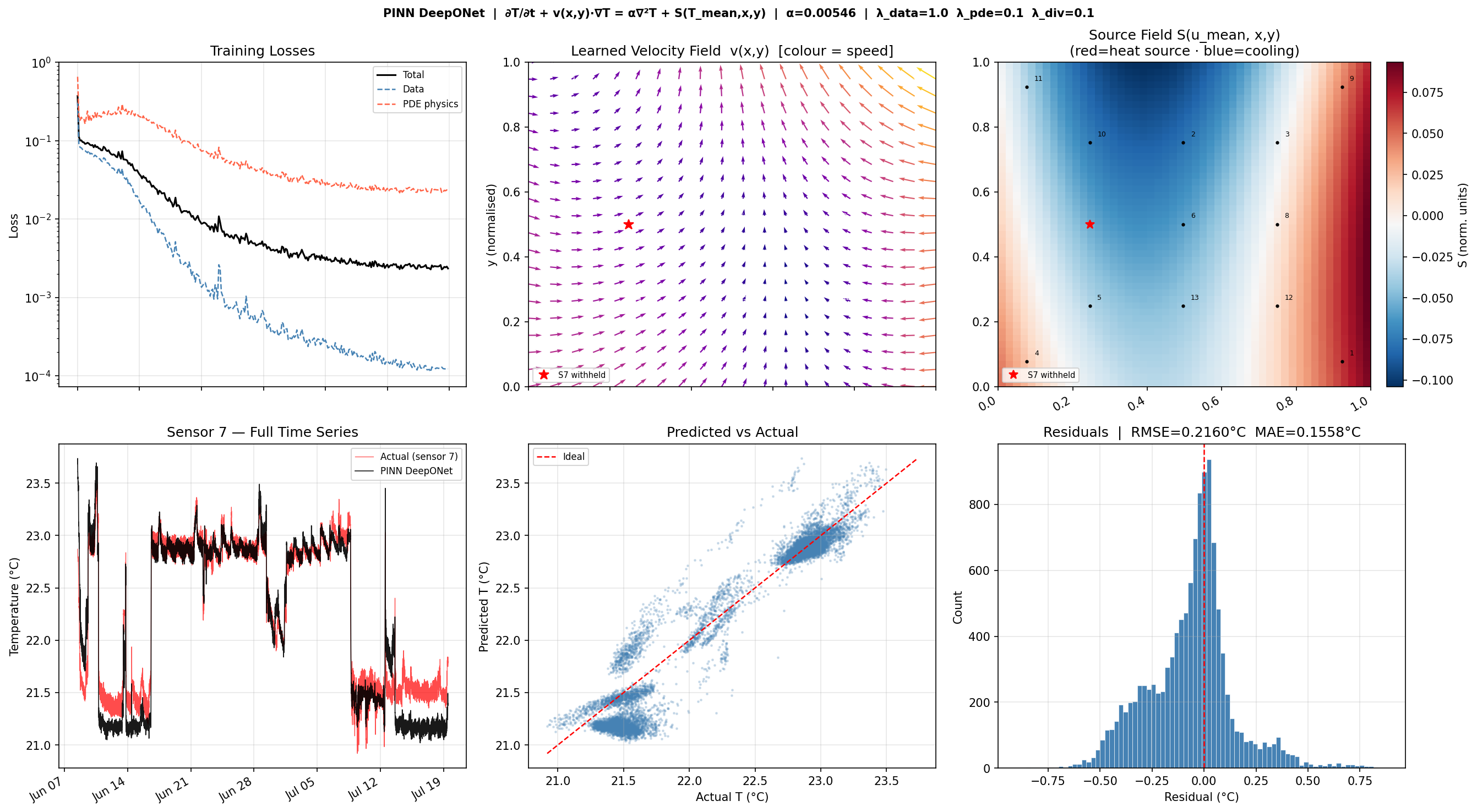
Figure 7 — Physics-Informed DeepONet Results.
Top row (left to right): training loss curves showing the data loss (blue dashed)
and PDE physics loss (red dashed) converging together;
learned velocity field v(x, y) as a quiver plot coloured by speed — arrows reflect
a leftward circulation pattern consistent with AC-driven airflow;
learned source field S(T̄, x, y) at mean thermal state showing a warm region
(red) on the right side of the room and a cooling zone (blue) on the left,
consistent with a localised heat source near sensors 1 and 9.
Bottom row: full time-series reconstruction of withheld Sensor 7 (α = 0.00546,
RMSE = 0.2160°C, MAE = 0.1558°C); predicted vs. actual scatter; residual histogram.
This result uses the SIREN trunk at ω₀ = 5 and mean-temperature-only source context.
The additional boundary condition losses (no-slip, Neumann, L1 sparsity) are implemented
in the code and will further constrain the velocity and source fields in the next training run.
8
LSTM-PINN DeepONet
LSTM-Branch DeepONet with Advection-Diffusion PINN
The previous physics section used a snapshot MLP branch — it treated every timestep
independently, with no memory of how the room arrived at its current state.
This section upgrades the branch network to an LSTM encoder,
giving the model a 4-hour sliding window of sensor history,
and combines it with a richer Advection-Diffusion-Source PDE
that simultaneously learns the air-velocity field, thermal diffusivity, and
spatial heat sources from data.
Why replace the snapshot branch with an LSTM?
A plain MLP branch encodes only the current sensor snapshot — it has no memory of
recent occupancy ramps, AC cycles, or thermal inertia.
An LSTM branch encodes the full trajectory of how the room got to its current
thermal state. This matters for two reasons:
∂T/∂t is estimated from consecutive LSTM embeddings whose hidden state
already reflects recent history — not just an instantaneous finite difference.
The velocity field v(x,y) is fitted against a model that already understands
directionality-over-time, so it converges to more physically plausible circulation patterns.
Architecture Overview
BRANCH NET — LSTM ENCODER ├─ Input: sliding window of 12 sensor temperatures over 48 timesteps (4 h) │ Shape: (batch, seq=48, n_sensors=12) ├─ LSTM: hidden=128, layers=2, dropout=0.1 between layers ├─ Take last hidden state of final layer → (batch, 128) └─ Linear projection → (batch, p=128) branch embedding b
TRUNK NET — SIREN MLP ├─ Input: normalised spatial query point (x, y) ∈ [0,1]² ├─ SIREN layers: 2 → 128 → 128 → 128 → 128 → 128 (depth=4) │ activation: sin(ω₀ · Wx + b), ω₀ = 5 │ ω₀ reduced from 30 — thermal fields are smooth; │ large ω₀ causes ∇²T ~ ω₀² blow-up in the PDE residual └─ Final linear layer (no sin) → (batch, p=128) trunk embedding t
OUTPUT T̂(x,y,t) = b · t + bias (inner product + scalar bias)
Instead of the simple heat equation used earlier, this model enforces a full
advection-diffusion-source PDE at a set of collocation points every training step:
∂T/∂t + v(x,y) · ∇T = α ∇²T + S(Tmean, x, y)
Each term has a concrete physical role:
∂T/∂t — temporal rate of change, estimated by a finite difference between
the model output at window [t−48:t] and window [t−47:t+1].
The LSTM hidden state encodes history, so these consecutive embeddings capture genuine dynamics.
v(x,y) · ∇T — advective transport by the spatially-varying air-circulation field.
v_net is a shallow MLP (2→16→2) that outputs (vx, vy)
at any room location. A soft divergence-free penalty ‖∇·v‖² ≈ 0 encourages mass conservation.
α ∇²T — diffusion. α = exp(log_α) is learned end-to-end; it starts near
e−2 ≈ 0.135 (normalised units) and converges to the physically meaningful value.
S(Tmean, x, y) — spatially-varying source/sink conditioned on the
mean sensor temperature of the last window step only. Using only Tmean
(a single scalar) as temporal context prevents the network from absorbing the full PDE residual
as a fudge factor. An L1 sparsity penalty forces S to localise into small distinct regions
(like real AC vents or equipment racks).
Derivative Computation
∂T/∂t (finite difference over LSTM windows) dT_dt = [ model(seq[t-48:t], xy) − model(seq[t-47:t+1], xy) ] / Δt Both sequences share the same spatial coords; only the LSTM history shifts by one step.
∇T (1st-order autograd through SIREN trunk) grad1 = ∂T̂/∂(x,y) via torch.autograd.grad with create_graph=True
∇²T (Laplacian via 2nd-order autograd) d²T/dx² = ∂(dT/dx)/∂x d²T/dy² = ∂(dT/dy)/∂y Laplacian = d²T/dx² + d²T/dy² SIREN activations (sin) have non-vanishing 2nd derivatives — this is why ReLU/Tanh trunks fail: their Laplacians are zero or extremely sparse.
Boundary Conditions
Four physics-motivated boundary conditions are enforced at 64 sampled wall points per edge
(256 total) each training iteration:
No-slip (Fix 1) — v(xwall) = 0.
Air velocity is zero at solid walls; penalised as ‖v_wall‖².
Neumann thermal BC (Fix 4) — ∂T/∂n = 0 at each wall (insulated boundary).
The normal gradient is extracted from autograd: ∂T/∂y for bottom/top walls,
∂T/∂x for left/right walls.
Divergence-free penalty (λ_div) — ‖∂vx/∂x + ∂vy/∂y‖²
encourages mass conservation throughout the domain (not just at walls).
Each training step draws 512 collocation points using a mixed strategy:
half (256) from the actual sensor locations (high-information zones), half (256) uniformly
random from the room interior [0,1]². This ensures the PDE residual is enforced both
where data is dense and in sparsely covered regions.
Loss Function
TOTAL LOSS L = λ_data · MSE_data + λ_pde · ( MSE_pde + λ_div · MSE_div + λ_noslip · MSE_noslip + λ_sparse · L1_source + λ_neumann · MSE_neumann )
HYPER-PARAMETERS λ_data = 1.0 (primary data-fitting objective) λ_pde = 0.1 (physics regularisation — strong enough without overwhelming data) λ_div = 0.1 (divergence-free penalty on v_net) λ_noslip = 0.1 (no-slip BC at walls) λ_sparse = 0.001 (L1 sparsity on source field) λ_neumann= 0.1 (Neumann ∂T/∂n = 0 at walls)
HARDWARE Auto-detects: Apple MPS → CUDA → CPU (MPS used on Mac M-series)
CHECKPOINTING Best epoch saved to deeponet_lstm_pinn_best.pth (lowest total loss) Final model saved to deeponet_lstm_pinn.pth
Withheld-Sensor Evaluation (Sensor 7)
Sensor 7 (location: x=1.92 m, y=3.91 m) is completely excluded from training —
it does not appear in the branch input, in the data loss, or in the collocation set.
After training, the model is queried at the sensor 7 coordinates for every valid timestep
and the prediction is compared against the true sensor 7 readings.
This tests spatial generalisation: the model must reconstruct temperature at an
unobserved location purely from the physics constraints and the 12 surrounding sensors.
Inference uses 512-sample chunks over the full time series
(first 48 timesteps are excluded as LSTM warm-up).
Predictions are de-normalised with the global mean and standard deviation from training.
Visualised Results
The 6-panel result figure provides a complete diagnostic view of the trained model:
Training losses (log scale) — total, data, and PDE physics components over 300 epochs.
Learned velocity field v(x,y) — quiver plot coloured by speed; shows the
air-circulation pattern the model discovered. Sensor positions are overlaid; sensor 7 (withheld) is
marked with a red star.
Source field S(Tmean, x, y) — heatmap of the learned heat source/sink
distribution (red = heating, blue = cooling) at the mean thermal state.
Sensor 7 full time series — predicted vs actual temperature over the 40-day dataset
(first 48 steps skipped for LSTM warm-up).
Predicted vs Actual scatter — ideal line in red; clustering around the diagonal
indicates low bias.
Residual histogram — centred near zero with RMSE and MAE annotations.
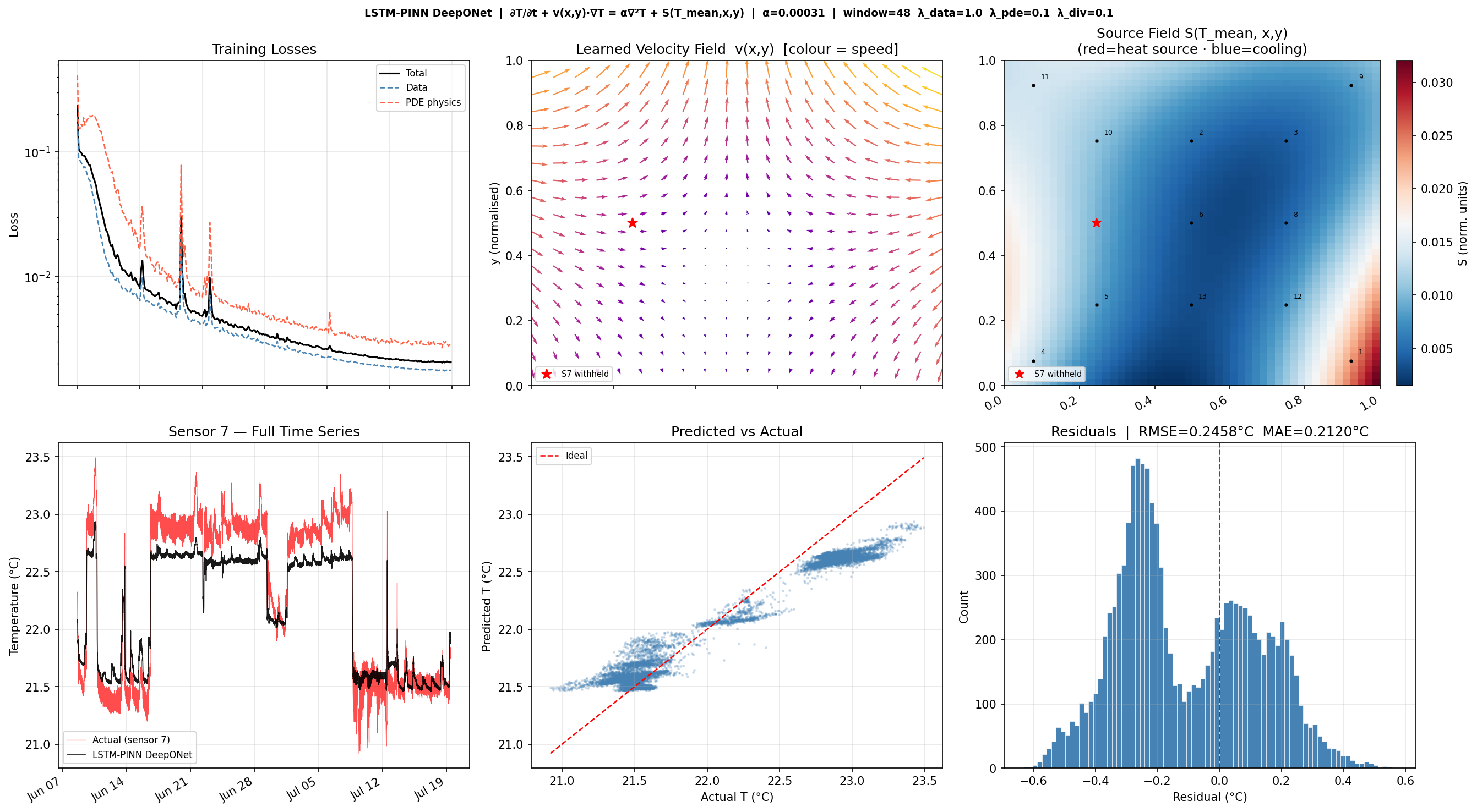
Figure 8-1 — LSTM-PINN DeepONet Diagnostic (6 Panels).
Top row (left to right): training loss curves (total, data, PDE physics) on a log scale;
learned spatially-varying velocity field v(x,y) from v_net — colour encodes flow speed,
sensor locations shown as white dots, withheld sensor 7 as a red star;
source/sink field S(Tmean, x, y) from source_net — red regions indicate
net heat input, blue regions net cooling.
Bottom row: full 40-day time-series reconstruction of withheld sensor 7 (predicted vs actual);
predicted vs actual scatter plot; residual histogram with RMSE and MAE.
Sensor 7 is excluded entirely from training — the reconstruction is driven purely by
physics constraints and the 12 surrounding sensors.
Learned Physics Parameters
After training the model reports the following learned PDE parameters:
Thermal diffusivity α — a single positive scalar (learned in log-space to
ensure positivity). The converged value reflects the effective thermal diffusivity of
the room in normalised units.
Velocity at each sensor location — (vx, vy) and speed
printed per sensor, giving a point-sample of the learned circulation field.
Key Improvements over the Snapshot PINN (Section 7)
The LSTM-PINN model differs from Section 7 in three fundamental ways:
Temporal memory: the LSTM branch encodes a 4-hour history of all 12 sensors;
the Section 7 branch encoded only the current snapshot.
Richer PDE: full advection + diffusion + spatially-varying source vs. a
simpler heat equation with learned α only.
Additional boundary conditions: no-slip for velocity, Neumann for temperature,
and L1 source sparsity are all active — physically grounding the sub-networks and
preventing unphysical solutions.
9
Uncertainty Quantification
Spatial Uncertainty Maps
Knowing how well the model knows the temperature at each room location is as important as
the prediction itself. A model that is confident everywhere — even where sensor coverage is sparse —
cannot be trusted for decision making (e.g. HVAC placement, fault detection).
We extend DeepONet to output both a mean prediction and a
predictive variance at every queried location.
What is Uncertainty Quantification?
Uncertainty quantification (UQ) means estimating not just a single prediction value but
also a confidence measure for that prediction. In a probabilistic neural network,
the model outputs the parameters of a probability distribution — here a Gaussian with
mean μ and variance σ² — instead of a single number.
A high σ² at a location signals that the model lacks confidence there,
typically because no training sensor is nearby. This spatial uncertainty can guide
decisions such as where to add new sensors to maximally reduce overall uncertainty.
Probabilistic DeepONet Architecture
PROBABILISTIC BRANCH NET ├─ Input: 13 sensor temperatures (all sensors used — no withholding) ├─ MLP: 13 → 128 → 128 → 128 → 2p (double output width) ├─ Split output into two halves: │ b_mean ∈ ℝp (mean latent) │ b_logvar ∈ ℝp (log-variance latent)
TRAINING LOSS Gaussian NLL: L = Σ [ log σ² + (T_true − μ)² / σ² ] The model is penalised for both inaccurate means and mis-calibrated variances.
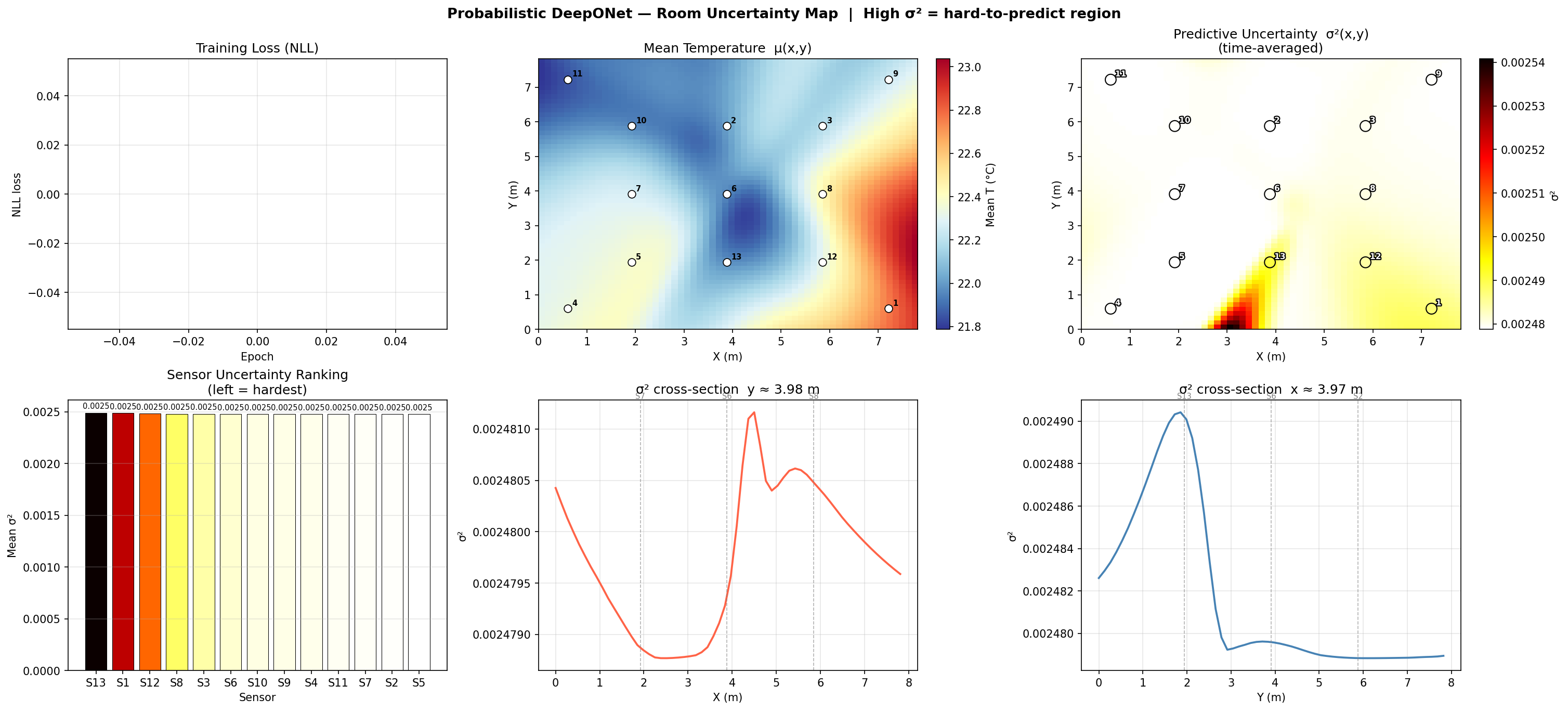
Full-Coverage Uncertainty Map
In the first experiment all 13 sensors are used as branch inputs. After training,
we query the model on a dense grid spanning the entire room and plot the predicted
variance σ² at each grid point as a heatmap.
Regions with low σ² are well-constrained by nearby sensors;
regions with high σ² represent locations the model is uncertain about.
Figure 9-1 — Predictive Uncertainty Map (All 13 Sensors). Spatial heatmap of predicted variance σ² across the room when all sensors are active. Low uncertainty near sensor locations, elevated uncertainty in corners and areas with sparse coverage.
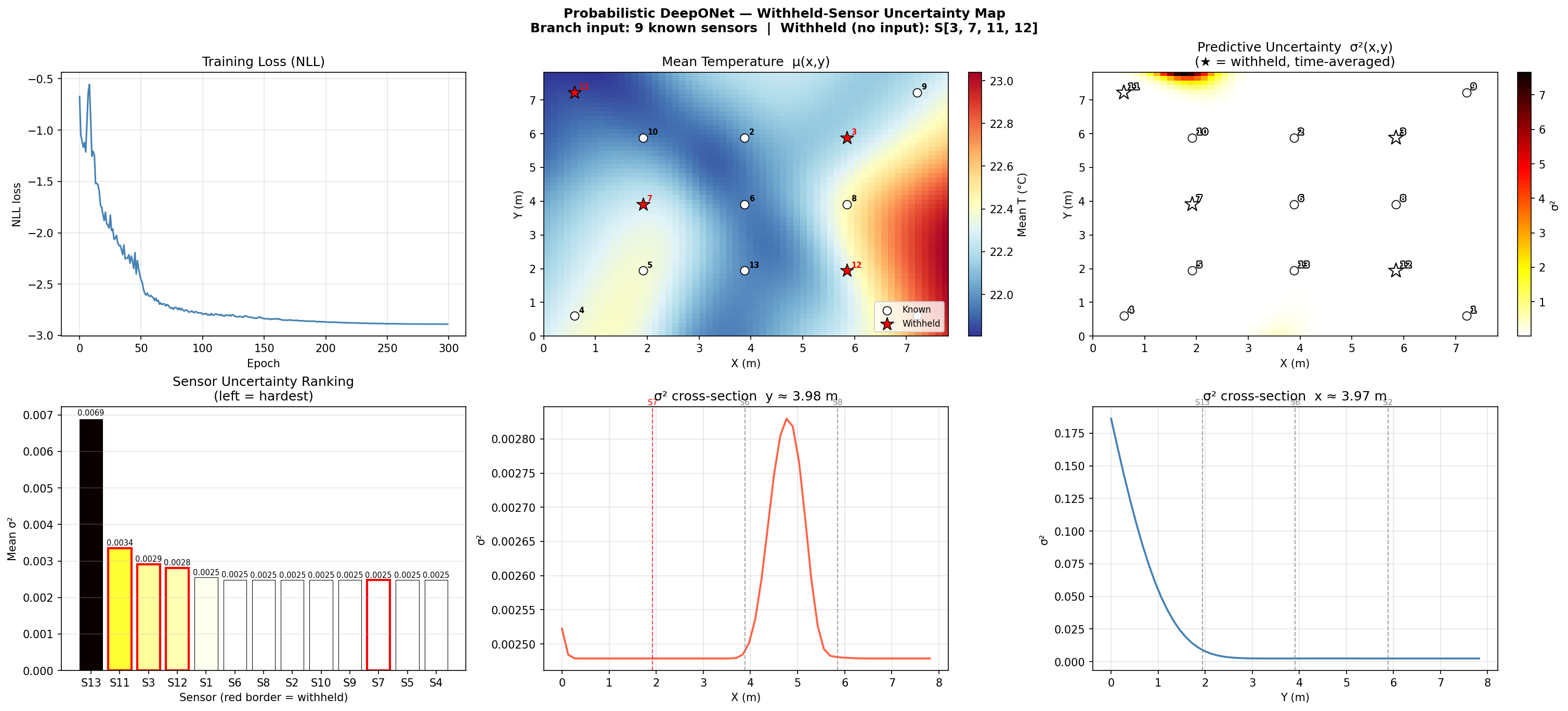
Uncertainty with Withheld Sensors
In the second experiment, 4 sensors are removed from the branch input,
simulating sensor failure or a sparser deployment.
The model receives only 9 sensor readings at inference time.
We expect σ² to spike at — or near — the withheld sensor locations,
since the model now has no direct information about those zones.
Figure 9-2 — Predictive Uncertainty Map (4 Sensors Withheld). Removing 4 sensors from the branch input causes σ² to rise at their locations, confirming the model correctly identifies its own ignorance. This property can be used to guide optimal sensor placement.
Practical Application
The uncertainty map answers the question: "If I can only afford N sensors, where should I place them?"
By iteratively adding a virtual sensor at the highest-σ² grid point and re-evaluating,
one can derive a greedy optimal sensor placement strategy purely from the trained probabilistic model —
no additional data collection required.
After the early single-sensor experiments above, the project was refactored into a cleaner
masked-reconstruction pipeline focused on Lab 1 at 5-minute resolution.
The newer versions move from a temperature-only baseline to a joint temperature + humidity model,
then to targeted sparsity tests and finally to a minimal active sensor study.
Across all newer versions, the branch input uses an explicit observed/missing mask,
test windows remain blocked in time, and evaluation is reported under controlled masking protocols.
Repository Layout for These Runs
Data files live under ./data, model code under ./deepOnet, and run outputs under
./deepOnet/runs. On GitHub, the multi-output run is stored under
lab1data_v0.2.2, the targeted sparsity run for DeepONet v0.3.2
is stored under lab1data_v0.3.1, and the sensor-importance study is stored under
lab1data_v0.4.1.
What Changed in the New Pipeline
The original single-target experiments were consolidated into a single reproducible workflow.
Missing sensors are no longer represented only by zero-fill; instead the model also receives an
explicit observed/missing mask. Later versions add joint temperature-humidity outputs,
early stopping, structured masking protocols, and sensor-subset search.
How These New Models Are Evaluated
Every evaluation masks the target sensor and varies how many additional sensors are hidden.
The analysis now goes beyond random masking: we also test central removal, perimeter removal,
spread-out removal, and leave-only-k-active subsets to understand not just how many
sensors matter, but also which ones matter most.
Version v0.1 — Temperature-Only Masked Reconstruction Baseline
The first consolidated baseline predicts temperature only and evaluates how well the model
reconstructs masked sensors from the remaining Lab 1 measurements. This version established the new
train/validation/test workflow and showed that the model was already strong at low masking levels,
but still fragile when too many sensors were removed.
Masked Total
Variable
RMSE
MAE
R²
1
Temperature
0.1253
0.1000
0.9596
3
Temperature
0.1699
0.1306
0.8965
6
Temperature
0.4045
0.3283
0.3795
Takeaway from v0.1
The baseline worked well when only a few sensors were missing, but performance collapsed at
6 masked sensors. This motivated the next redesign: joint temperature-humidity training,
wider masking during training, and stronger control over evaluation protocols.
Version v0.2.2 — Joint Temperature + Humidity Reconstruction
The next major upgrade predicts temperature and relative humidity together in a single model.
This version also introduced early stopping and a wider masking distribution during training.
The result was a large jump in robustness: the joint model remained accurate not only at low masking,
but even in the severe-sparsity regime.
Masked Total
Temp RMSE
Temp R²
Humidity RMSE
Humidity R²
1
0.0975
0.9616
0.4214
0.9845
3
0.1067
0.9564
0.4651
0.9809
6
0.1334
0.9454
0.5709
0.9725
9
0.2182
0.8659
0.9856
0.9241
12
0.5103
0.3652
2.8315
0.4482
Takeaway from v0.2.2
The multi-output model stayed strong all the way to 9 masked sensors, and only really broke down
at 12 masked sensors. This was the point where the question shifted from
“can the model reconstruct missing sensors?” to “which remaining sensors are the most valuable?”
Version v0.3.2 — Targeted Sparsity Characterisation
To probe the sparsity boundary more carefully, v0.3.2 evaluated structured masking protocols for
8, 9, 10, 11, and 12 masked sensors. Instead of only using random masks, we also tested
central removal, perimeter removal, spatially spread removal, and leave-only-k-active subsets.
This reveals whether performance depends only on the number of active sensors or also on their spatial arrangement.
Masked Total
Best Protocol
Temp R²
Humidity R²
Weakest Protocol
Temp R²
Humidity R²
8
Spread removed / Perimeter removed
0.9332
0.9674
Central removed
0.9019
0.9551
9
Spread removed / Perimeter removed
0.9255
0.9621
Central removed
0.8897
0.9520
10
Spread removed
0.9239
0.9553
Central removed / Random
0.9000
0.9523
11
Active central diagonal / Perimeter removed
0.9042
0.9535
Corner diagonal only / Random
0.8715
0.9399
12
Spread removed
0.8643
0.9289
Center one only
0.6350
0.8103
Main Interpretation from v0.3.2
Even with 11 masked sensors, the model still performs fairly well under multiple protocols.
The real performance cliff appears at 12 masked sensors, where the exact spatial arrangement of the
remaining sensors becomes decisive. Spread-out coverage is much more informative than relying on a single central point.
Version v0.4.1 — Sensor Importance and Minimal Active Sets
Once the sparsity boundary was understood, the next step was to determine which sensors are actually necessary.
Version v0.4.1 adds three analyses: a one-at-a-time drop test, a greedy backward elimination path,
and an exhaustive search over all active subsets of size 1, 2, and 3.
The results show that the room contains a large amount of redundancy and that only a small,
well-placed subset of sensors is enough for strong reconstruction.
Most Expendable Sensors
In the single-sensor drop study, removing sensors 9, 7, 6, or 10
had the smallest effect on the overall score. This suggests these locations are more redundant than the others.
Most Informative Sensors
Sensors 5, 8, and 3 are the hardest to remove without hurting performance.
Sensor 5 is especially important: it survives until the very end of the backward elimination path
and is also the best single active sensor in the exhaustive search.
Main Practical Result
The best 2-sensor set already delivers strong reconstruction, and the best 3-sensor set
comes surprisingly close to the full 13-sensor reference. In other words: the minimal useful set is much smaller than expected.
Active Count
Best Active Sensors
Composite Score
Temp R²
Humidity R²
1
[5]
0.8391
0.8140
0.8642
2
[5, 8]
0.9334
0.9157
0.9512
3
[2, 5, 8]
0.9445
0.9271
0.9618
BACKWARD ELIMINATION ORDER 9 → 7 → 1 → 13 → 12 → 4 → 6 → 10 → 3 → 11 → 2 → 8 Sensor 5 is the final remaining sensor.
BEST FULL-REFERENCE PERFORMANCE All 13 active sensors: R²temperature = 0.9384 | R²humidity = 0.9745 Best 3-sensor subset: R²temperature = 0.9271 | R²humidity = 0.9618 Best 2-sensor subset: R²temperature = 0.9157 | R²humidity = 0.9512 Best 1-sensor subset: R²temperature = 0.8140 | R²humidity = 0.8642
Current Conclusion
The newer DeepONet pipeline shows that Lab 1 is highly redundant spatially.
Strong temperature-humidity reconstruction is possible with only 2–3 strategically placed sensors,
and even a single well-chosen sensor can recover much of the room state.
The next natural step is transfer: testing whether a model trained on Lab 1 can adapt to Lab 2.
11
Final Model Design
Chosen Final Model (v0.5.3) — Why It Won and How It Works
The Step-5 architecture benchmark compared six closely related models: the compact comparison baseline (v0.5.1),
a wider snapshot model (v0.5.2), a deeper snapshot model (v0.5.3), a short-history LSTM branch model (v0.5.4),
a deep+wide model (v0.5.5), and a deep+GELU variant (v0.5.6). The strongest average score was achieved by the
LSTM model v0.5.4, but only by a tiny margin over v0.5.3. Because the gain was negligible while the architecture
was more complex, the project standardised on v0.5.3: the deep snapshot DeepONet with explicit masking.
Model
Main Change
Mean R² (all comparison protocols)
Decision
v0.5.1
Compact benchmark reference
0.9195
Baseline only
v0.5.2
Wider snapshot MLP
0.9227
Small gain
v0.5.3
Deeper snapshot MLP (depth = 6)
0.9301
Chosen final model
v0.5.4
Short-window LSTM branch
0.9310
Tiny edge, but more complex
v0.5.5
Deep + wide
No clear gain
Rejected
v0.5.6
Deep + GELU
No clear gain
Rejected
Selection Logic
Step 5 showed that depth mattered more than width, and that moving from tanh to GELU did not unlock a better model.
Because v0.5.3 stayed essentially tied with v0.5.4 while keeping a simpler operator structure and a cheaper transfer pipeline,
it became the model carried forward into the Lab1→Lab2 transfer study.
Architecture
INPUTS Branch values: 13 sensors × 2 channels (temperature, humidity) = 26 scalar values Observed-mask: 13 binary indicators showing which sensors are visible = 13 Trunk input: query coordinate (x, y), normalised by room width and height = 2
OUTPUT For each variable, prediction = inner product(branch, trunk) + learned bias Final output dimension = 2 (temperature and humidity at the queried coordinate)
Why Keep the Trunk This Simple?
The trunk sees only normalised coordinates. That is intentional: all temporal and sensor-state information lives in the branch,
while the trunk learns a purely spatial basis. This keeps the operator decomposition clean and makes transfer to a new room easier
to interpret because geometry enters only through the coordinate system.
Why Keep the Snapshot Branch?
The LSTM branch gave only a tiny average gain. The project therefore chose the deeper snapshot branch instead: it captures the
spatial state very well, remains fast, and is easier to fine-tune in transfer experiments because there is no recurrent state to adapt.
Data Loading and Normalisation Strategy
The data pipeline is deliberately conservative to avoid leakage. For each run, the code reads the common time file
Time_5min.xlsx plus one file per variable (Temperature_5min.xlsx and Humidity_5min.xlsx),
extracts the 13 sensor columns, and stacks them into a tensor of shape [time, sensor, variable].
Every raw value is divided by 100 before modelling so that the two channels live on similar numeric scales.
Any timestep containing a NaN anywhere in the full sensor-variable tensor is dropped completely, which guarantees that the operator
never sees partially missing raw data before masking is applied on purpose.
NORMALISATION PIPELINE 1. Read all sensors for all selected variables at 5-minute resolution 2. Remove any timestep with a NaN in any sensor / variable entry 3. Build the blocked train / val / test split first 4. Compute one global mean and one global std per variable from the training split only 5. Apply z-score normalisation to all splits using those training-only statistics 6. Denormalise back to physical units only for evaluation and reporting
Subtle but Important Detail
The mean and standard deviation are computed across all training timesteps and all 13 sensors for each variable.
This means the model is not trying to learn separate sensor-wise calibration offsets inside the network. Instead, the network sees a
common standardised variable space and must learn spatial structure from the coordinates and masking pattern.
How Masking is Implemented
Earlier versions simply zero-filled missing sensors. That turned out to be ambiguous, because after z-score normalisation a value near zero
can also mean “this sensor is close to the mean.” The final design fixes that by feeding the model both the masked values and an
explicit observed/missing mask. During training, every sample chooses one target sensor and always hides it, then hides a random number of
additional sensors chosen uniformly between 1 and 12. The branch therefore sees a broad sparsity distribution during training rather than
only one carefully scripted masking level.
Always Hide the Target
Each sample is indexed by a timestep and a target sensor. The target sensor is always masked in the branch input and becomes the supervision target.
Random Extra Masks
Extra missing sensors are sampled from the remaining 12 sensors. This makes the operator robust to a wide range of sparse deployment regimes.
Observed-Mask Channel
The explicit 13-dimensional mask tells the network which zeros are true missingness and which are genuine near-mean standardised values.
Split Strategy: Benchmark vs. Transfer
The project uses two different blocked split policies for two different questions. In the architecture benchmark (v0.5.x), the model kept the
earlier blocked-window split so that all candidate architectures were compared under exactly the same conditions. Once the architecture was chosen,
the transfer study upgraded the split to a larger blocked design that is closer to a real held-out deployment scenario.
Stage
Purpose
Split Logic
Why
v0.5.x benchmark
Compare architectures fairly
Compact blocked validation and test windows inherited from the earlier pipeline
Preserves strict comparability with all previous Lab 1 runs
v0.6.1 transfer
Train final Lab 1 source model
Blocked 80/10/10 on Lab 1 using 6-hour windows
Provides a stronger held-out source split for transfer
v0.6.1 transfer
Adapt / test on Lab 2
Blocked 16/4/10 on Lab 2 (adapt-train / adapt-val / test)
Keeps a clean unseen Lab 2 test set while reserving a small adaptation budget
Optimisation Details
TRAINING SETUP Batch size: 4096 Optimiser: Adam Initial learning rate: 1e-3 Weight decay: 0 Scheduler: cosine annealing over the full epoch budget Max epochs: 150 Early stopping: patience = 20, min_delta = 1e-4 Model selection: save the best checkpoint on validation loss, evaluate that checkpoint only
What We Learned from Step 5
The project explicitly tested whether more width, recurrent temporal context, deeper+wide capacity, or GELU activations gave meaningful gains.
They did not. The practical sweet spot was the deep tanh snapshot model. That result is useful in itself: the bottleneck is not simply “make the
network bigger,” but rather choosing a masking formulation and split policy that expose the right reconstruction problem.
12
Transfer Learning
Lab 1 → Lab 2 Transfer (v0.6.1 Phase 1)
After selecting v0.5.3 as the final source architecture, the next question was whether the model learned anything that generalises beyond Lab 1.
Lab 2 is a different room with a different aspect ratio, different sensor geometry, different equipment layout, and a different air-conditioning structure.
In the source paper, LAB2 is described as having two thermal focal points due to its two AC outlets, so transfer is a genuine domain-shift test,
not just another split of the same room.
Phase 1 Transfer Modes
Phase 1 evaluates the two transfer endpoints: zero-shot (no Lab 2 training at all) and full fine-tuning
(adapt the entire network on a small blocked Lab 2 adaptation split with a lower learning rate).
Sensor Regimes
Instead of only testing all 13 sensors, the transfer study also evaluates sparse deployment regimes on Lab 2:
all 13 active sensors, a 5-sensor subset, and a 3-sensor subset. This separates true domain transfer from sheer sensor-count effects.
Phase 1 Results
Transfer Mode
Lab2 Protocol
Temp R²
Humidity R²
Main Interpretation
Zero-shot
All 13 active
0.9029
0.8710
Strong transfer without any Lab 2 training
Zero-shot
5 active
0.8929
0.8425
Still meaningful under sparse deployment
Zero-shot
3 active
0.9113
0.8705
Chosen 3-sensor subset was surprisingly informative
Full fine-tune
All 13 active
0.9854
0.9721
Closes almost the entire transfer gap
Full fine-tune
5 active
0.9816
0.9692
High-quality sparse transfer
Full fine-tune
3 active
0.9818
0.9633
Excellent adaptation even under strong sparsity
Main Transfer Takeaway
The source-trained Lab 1 model transfers to Lab 2 better than expected even zero-shot, and full fine-tuning becomes extremely strong.
For temperature, the fine-tuned Lab 2 model even reaches or exceeds the corresponding Lab 1 reference averages. This is strong evidence that the operator
is learning a transferable representation of indoor thermo-hygrometric structure rather than only memorising one room.
Why This Result Matters
A digital twin is most useful when it can be deployed to a room that was never part of training. The zero-shot result shows that the model already carries
non-trivial cross-room information. The fine-tuning result then answers the practical question: if zero-shot is not enough, a relatively small amount of new
Lab 2 data is sufficient to adapt the model into a high-quality room-specific surrogate.
Phase 2 (Ongoing)
The next transfer stage is now running. Phase 2 tests head-only and partial fine-tune adaptation across many Lab 2 sensor subsets,
focusing on 5, 3, and 2 active sensors. The goal is no longer just to show transfer works; it is to determine
how much adaptation capacity is needed and which sparse Lab 2 sensor layouts are most informative.
STEP 6 ROADMAP Phase 1: zero-shot + full fine-tune → completed Phase 2: head-only + partial fine-tune across many 5/3/2-sensor subsets → running Final question: what is the minimum Lab 2 adaptation budget and minimum sensor set needed for reliable transfer?
13
Transfer Adaptation Capacity
Lab 2 Adaptation Capacity — Zero-Shot, Head-Only, Partial, and Full Fine-Tune
The v0.7.1 pipeline unifies the full Lab 1 → Lab 2 transfer story in one comparable benchmark. Instead of evaluating different transfer modes on different protocol sets,
all modes are now measured on the same blocked Lab 2 split, the same selected sparse subsets, and the same reporting tables and figures.
This makes the comparison between zero-shot, head-only, partial fine-tune, and full fine-tune directly interpretable.
What changed in v0.7.1?
One single pipeline now handles Lab 1 pretraining, Lab 2 adaptation, sparse subset search, unified re-evaluation, and figure generation.
That removes the earlier mismatch between fixed v0.6.1 protocols and sampled v0.6.2 protocols.
What does Phase 2 answer?
Not only whether transfer works, but how much adaptation capacity is needed to recover high-quality Lab 2 performance under 5, 3, and 2 active-sensor regimes.
Mean R² by regime from the unified v0.7.1 benchmark
Regime
Zero-shot Temp R²
Head-only Temp R²
Partial FT Temp R²
Full FT Temp R²
Zero-shot Humidity R²
Head-only Humidity R²
Partial FT Humidity R²
Full FT Humidity R²
All 13 active
0.833
0.960
0.970
0.981
0.889
0.968
0.975
0.986
Top 5 mean (k=5)
0.825
0.956
0.968
0.978
0.876
0.965
0.973
0.984
Top 5 mean (k=3)
0.820
0.959
0.968
0.978
0.864
0.969
0.975
0.982
Top 5 mean (k=2)
0.808
0.952
0.963
0.974
0.865
0.964
0.969
0.978
Main v0.7.1 Takeaway
Zero-shot transfer is meaningful, head-only adaptation recovers most of the lost performance, partial fine-tuning improves further,
and full fine-tuning is the strongest overall mode. This ranking is stable across all-13 sensing and the selected sparse subsets, which is exactly what the final benchmark needed to show.
Important interpretation note
The LAB1 reference bars later on are a useful anchor, but they are not a strict upper bound for Lab 2. They come from a different room, with a different geometry and different test distribution.
So when the fully adapted Lab 2 model matches or slightly exceeds the Lab 1 reference in some summaries, that should be read as very strong target-domain performance, not as a contradiction.
14
Unified Benchmark
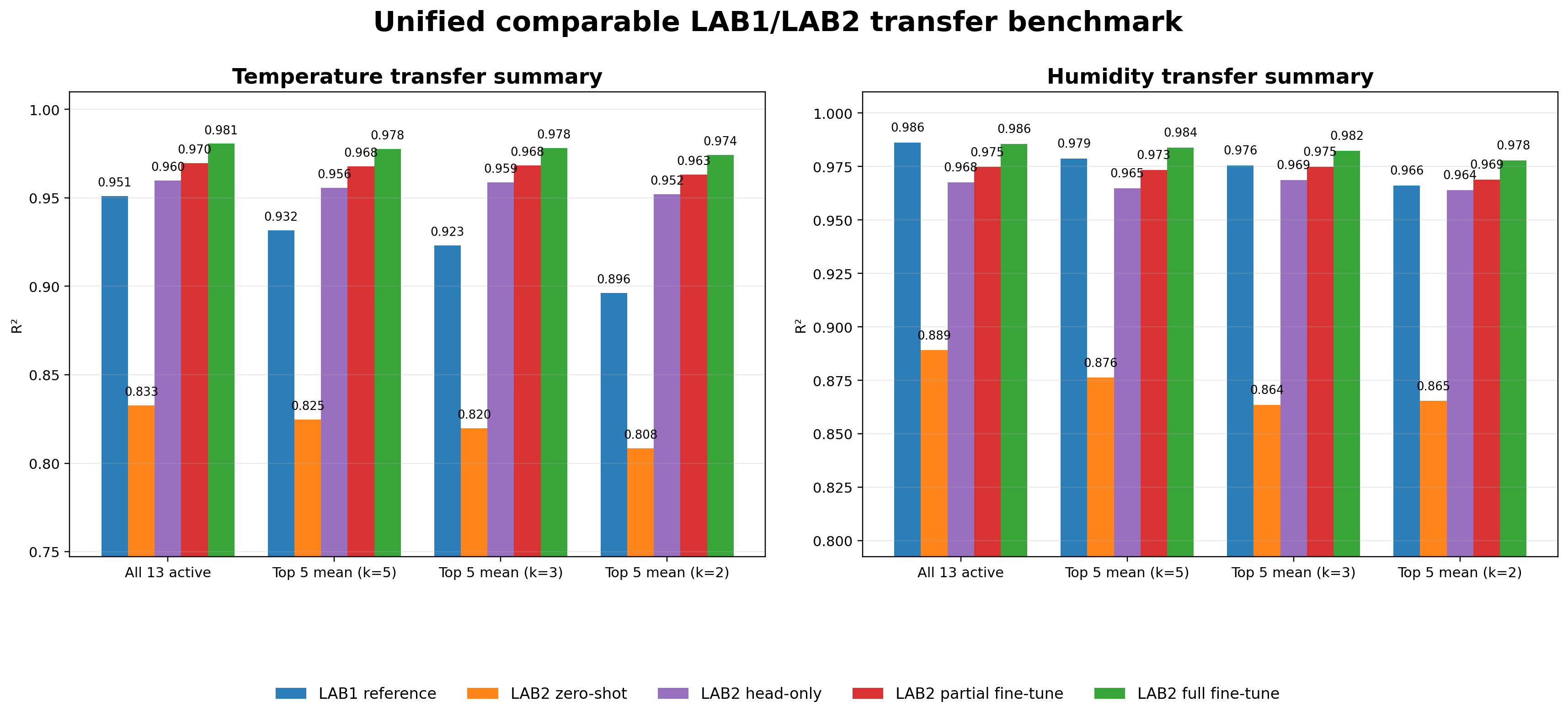
Unified LAB1/LAB2 Transfer Benchmark (v0.7.1)
The final website benchmark now uses the exact v0.7.1 outputs. The benchmark re-evaluates LAB1 reference, LAB2 zero-shot,
LAB2 head-only, LAB2 partial fine-tune, and LAB2 full fine-tune on a single shared protocol set:
all 13 active sensors, plus the top 5 subsets for k=5, k=3, and k=2 discovered from the head-only subset search.
This is the clean, directly comparable transfer benchmark that the final report and website were aiming for.
Unified comparable LAB1/LAB2 transfer benchmark. Mean R² values for temperature and humidity under the all-13 regime and the selected sparse subset regimes.
Zero-shot is already meaningful, head-only provides a strong lightweight adaptation baseline, partial fine-tuning improves further, and full fine-tuning performs best overall.
Headline numbers from the common benchmark
Regime
LAB1 Ref Temp R²
LAB2 Zero-shot Temp R²
LAB2 Head-only Temp R²
LAB2 Partial FT Temp R²
LAB2 Full FT Temp R²
LAB1 Ref Humidity R²
LAB2 Zero-shot Humidity R²
LAB2 Head-only Humidity R²
LAB2 Partial FT Humidity R²
LAB2 Full FT Humidity R²
All 13 active
0.951
0.833
0.960
0.970
0.981
0.986
0.889
0.968
0.975
0.986
Top 5 mean (k=5)
0.932
0.825
0.956
0.968
0.978
0.979
0.876
0.965
0.973
0.984
Top 5 mean (k=3)
0.923
0.820
0.959
0.968
0.978
0.976
0.864
0.969
0.975
0.982
Top 5 mean (k=2)
0.896
0.808
0.952
0.963
0.974
0.966
0.865
0.964
0.969
0.978
Why this section matters
This benchmark finally resolves the old comparability problem. Earlier versions mixed fixed protocols and sampled subset sweeps, which made direct transfer-mode comparison awkward.
In v0.7.1, every mode is scored on the same selected benchmark, so the conclusions are much more defensible.
Selected sparse subsets
The strongest sparse subsets were selected from the head-only search and then reused for the common benchmark. A practical pattern stands out immediately:
sensor 12 appears repeatedly, often together with sensors 2, 11, 1, 10, or 9.
That suggests the best sparse layouts are leveraging a few strategically informative locations rather than merely spreading sensors evenly across the room.
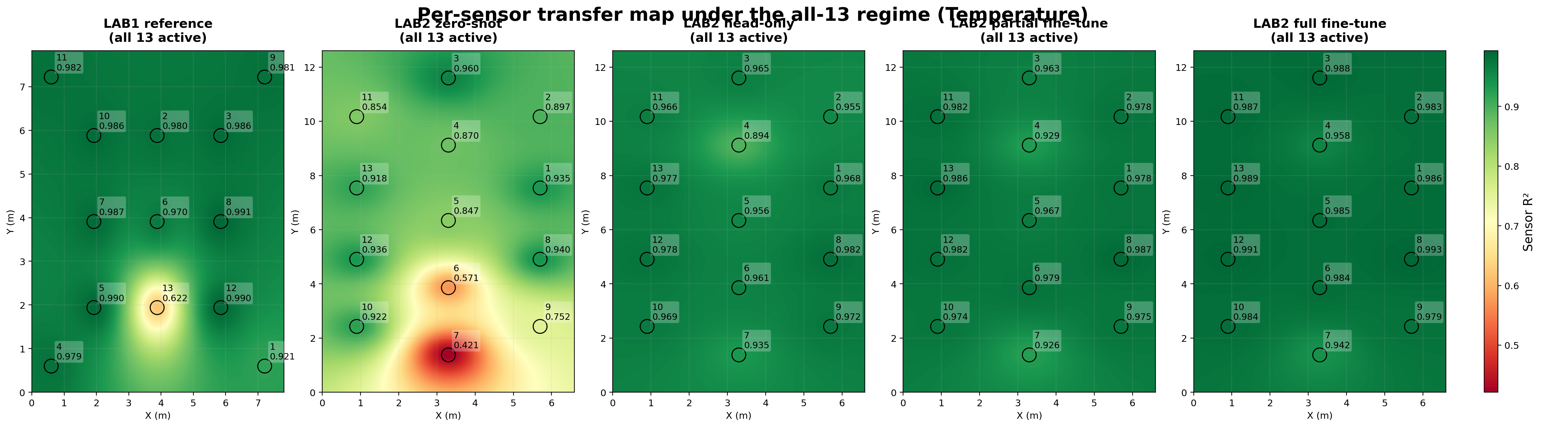
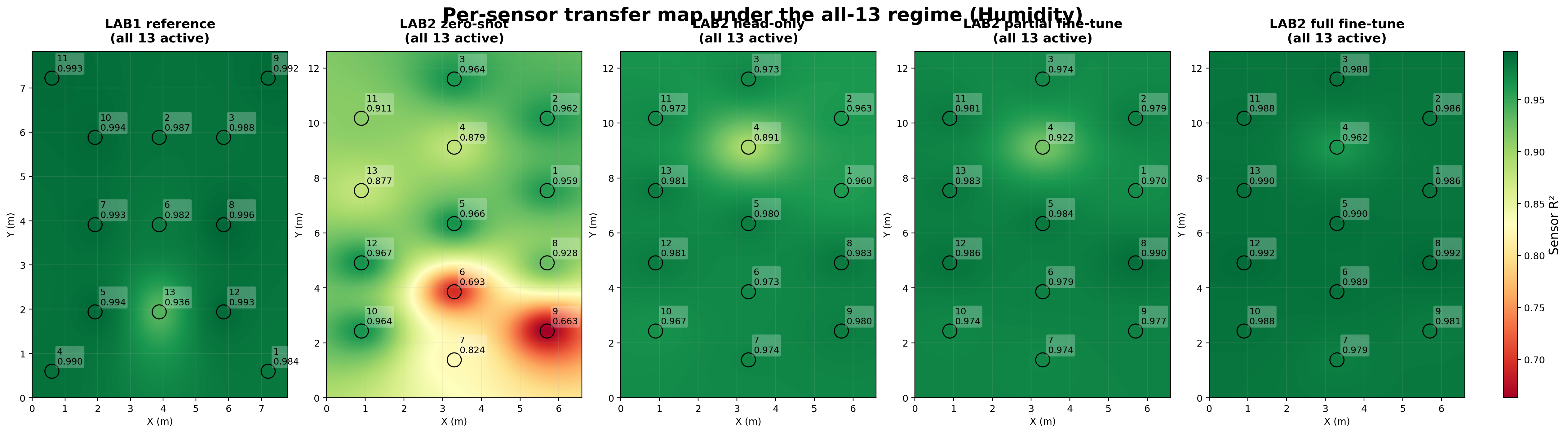
The all-13 maps make the spatial transfer story visible. In both temperature and humidity, the zero-shot errors are not uniform across the room; they are concentrated in a few difficult Lab 2 regions.
Head-only and partial fine-tuning correct most of those local failures, and full fine-tuning produces a nearly uniform high-R² map.
Per-sensor transfer map (temperature). The largest zero-shot temperature failures appear around sensors 7, 6, and 9, while head-only, partial fine-tuning, and especially full fine-tuning remove most of that local degradation.
Per-sensor transfer map (humidity). Humidity transfers slightly better than temperature in zero-shot, but the same pattern holds: the difficult regions are localised, and adaptation makes the spatial performance much more uniform across Lab 2.
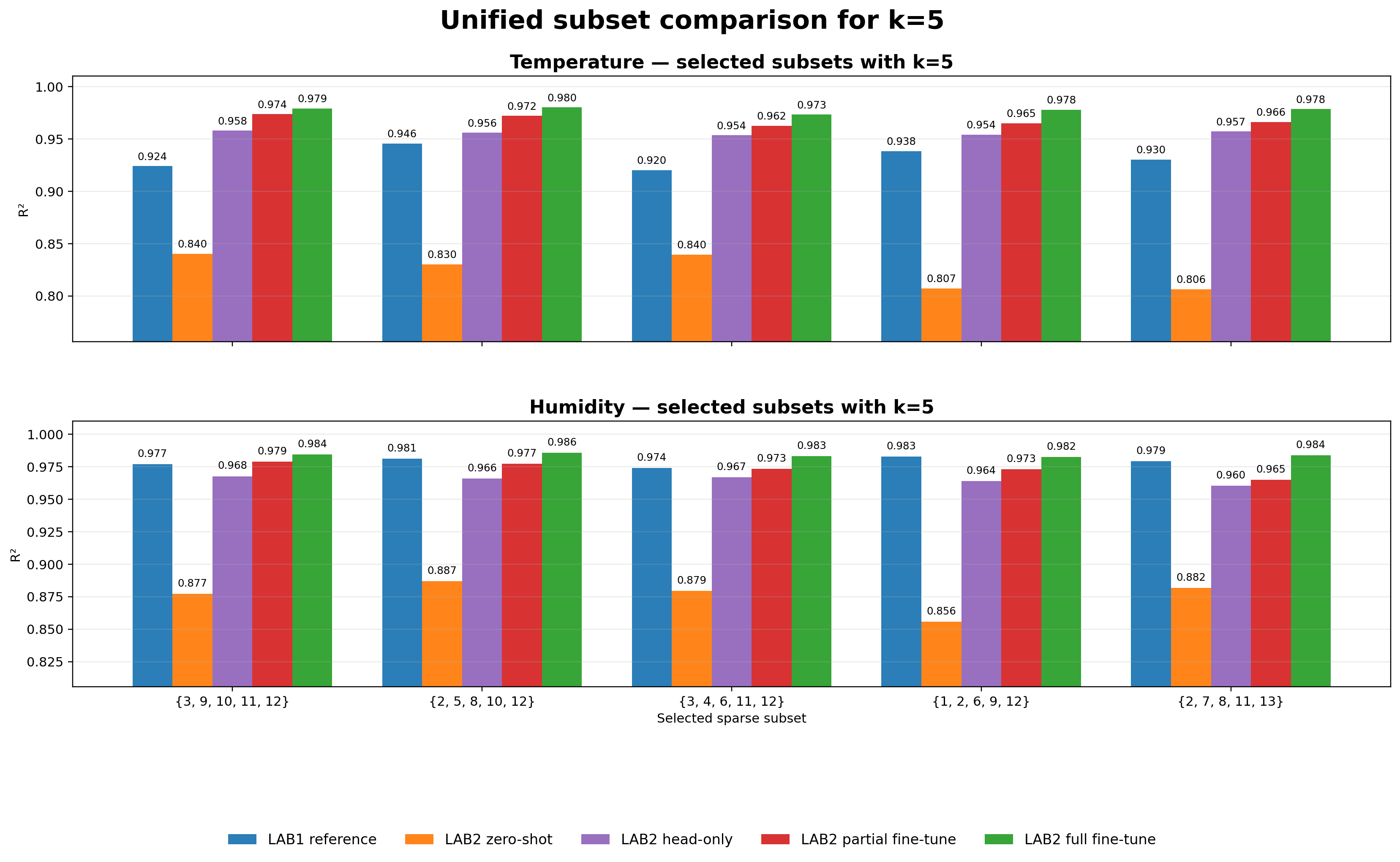
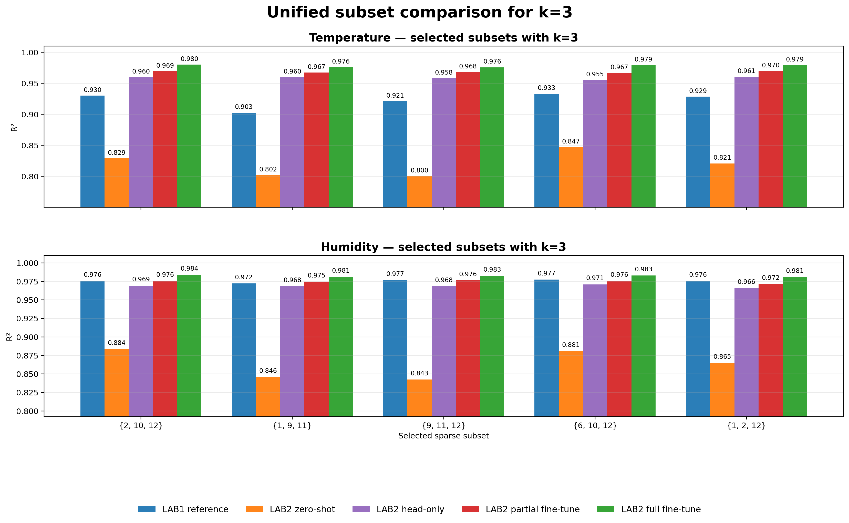
Sparse subset comparison figures
The next figures show the exact selected sparse subsets for k=5, k=3, and k=2. These are not averages over all possible subsets.
They are the strongest subsets discovered in the head-only search, re-evaluated under every transfer mode on the common benchmark.
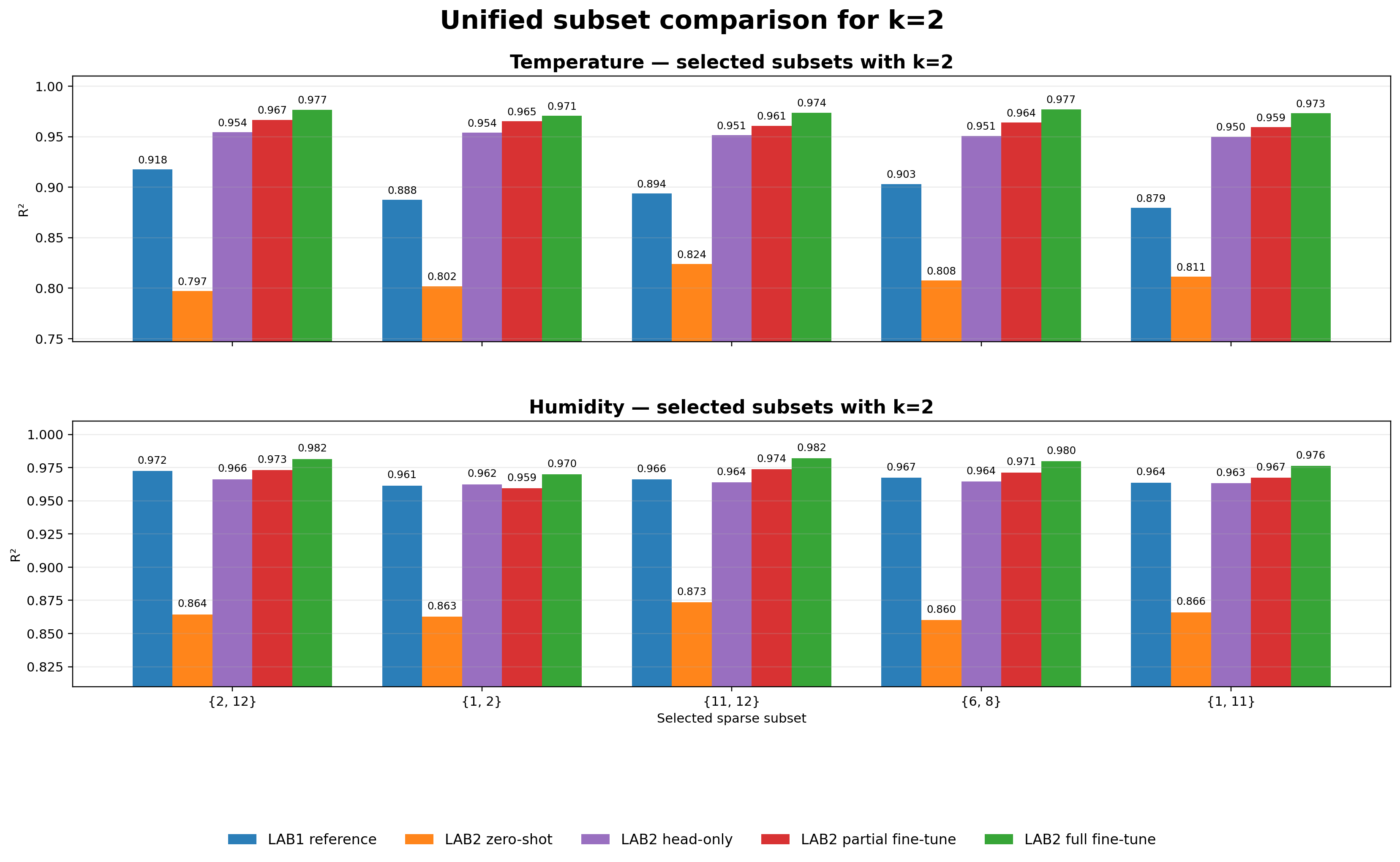
Selected subsets with k=5. Sparse transfer remains strong with only five active sensors. Head-only already recovers most of the zero-shot gap, partial fine-tuning improves further, and full fine-tuning remains the strongest overall mode.
Selected subsets with k=3. Even under only three active sensors, the transfer story is stable: zero-shot remains useful, adaptation closes a large portion of the gap, and full fine-tuning stays best.
Selected subsets with k=2. This is the strongest stress test in the benchmark. Despite only two active sensors, the adapted models still achieve very strong temperature and humidity reconstruction, especially under partial and full fine-tuning.
Example spatial field reconstructions
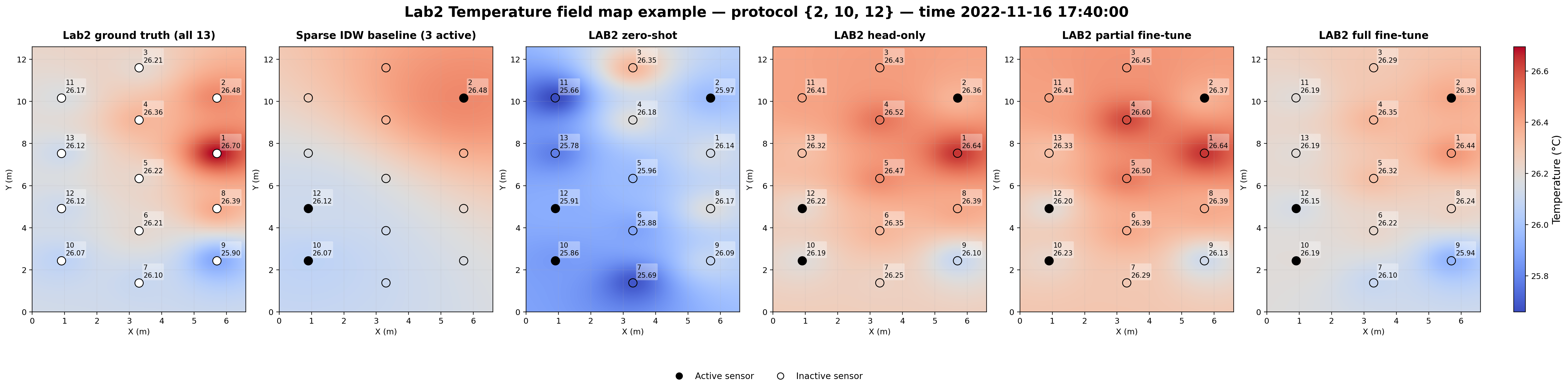
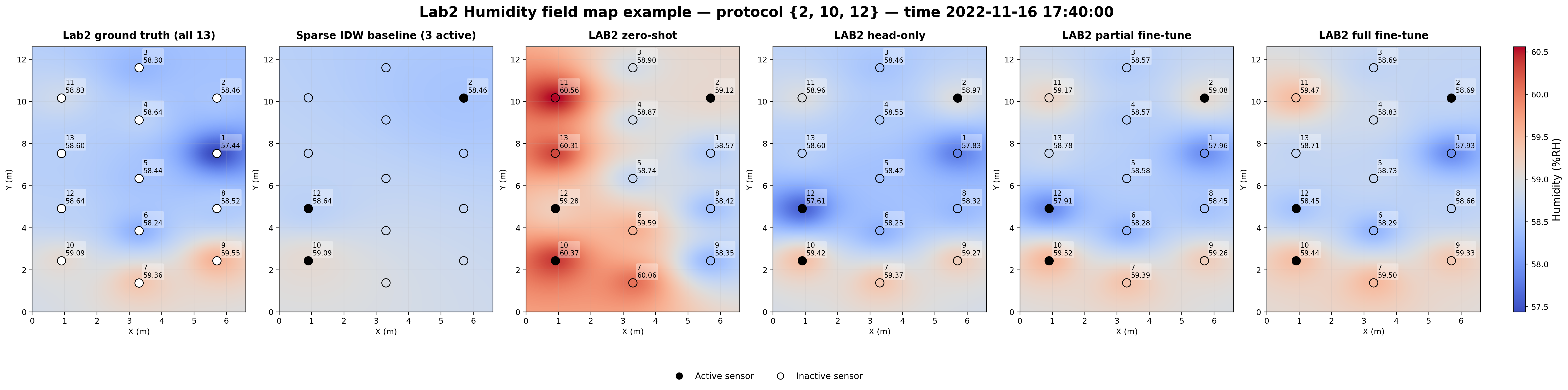
These example plots compare the Lab 2 ground truth, a sparse IDW baseline, and the DeepONet reconstructions under the different transfer modes for the same sparse protocol.
The IDW baseline is easy to interpret but visibly oversmooths the field. The adapted DeepONet models recover sharper and more realistic room structure from the same sparse sensor input.
Temperature field example. For protocol {2, 10, 12}, the sparse IDW baseline captures only a smooth approximation. Zero-shot reflects the room structure but with local distortions, while the adapted DeepONet variants move much closer to the ground-truth thermal field.
Humidity field example. The same comparison for humidity. The adapted operator reconstructs more plausible moist/dry regions than the sparse IDW baseline, particularly near the local extrema.
Current scope vs. next step
The current pipeline reconstructs dense temperature and humidity fields. A separate thermal comfort model is still the next layer to add on top of these reconstructed fields; it is not yet part of the current benchmark outputs.